Main workshop (primer)
Self-introduction
Kozo Nishida, RIKEN, Japan
- A member of Bioconductor Community Advisory Board (CAB)
- Author of a Bioconductor package based on RCy3 (transomics2cytoscape)
- Cytoscape community contributor (Google Summer of Code, Google Season of Docs)
- Author of KEGGscape Cytoscape App
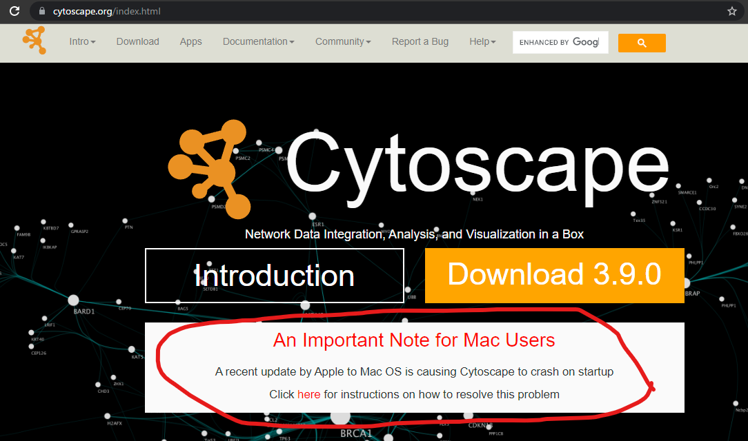
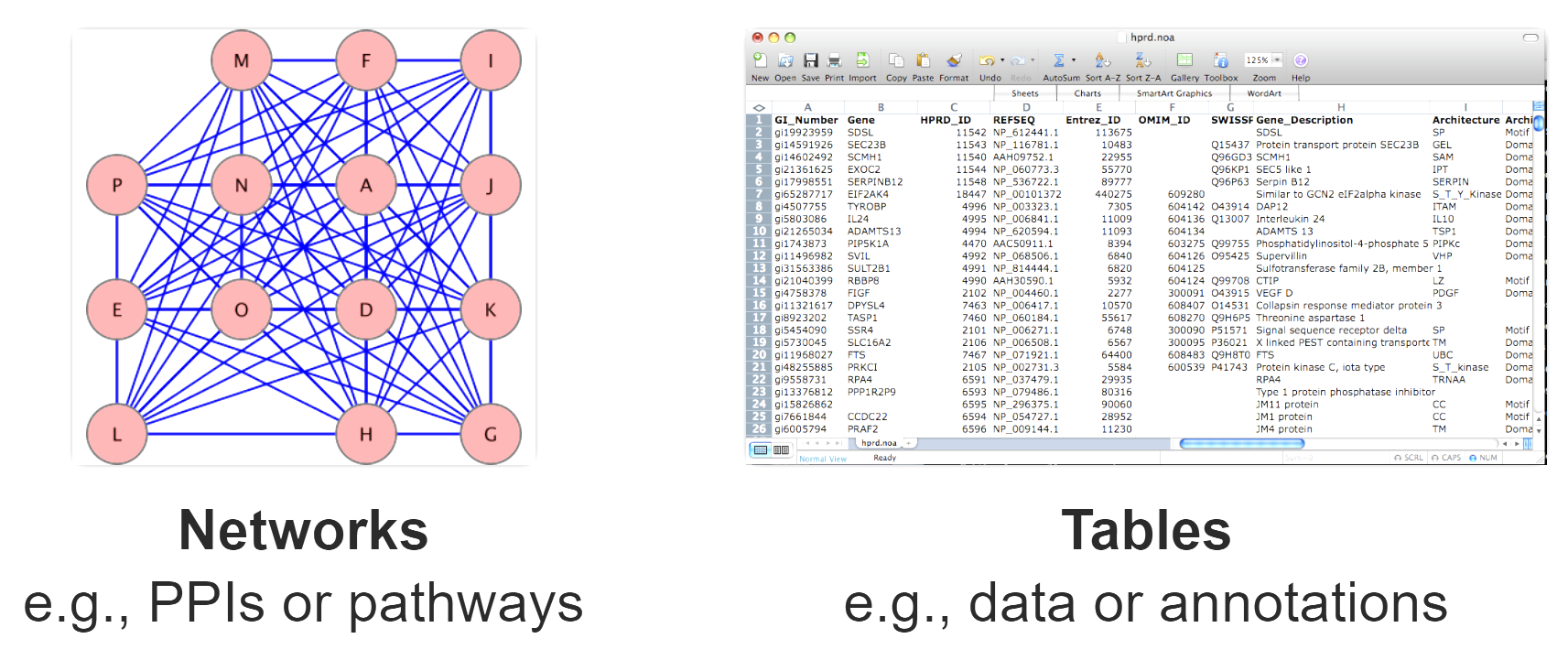
What is Cytoscape?
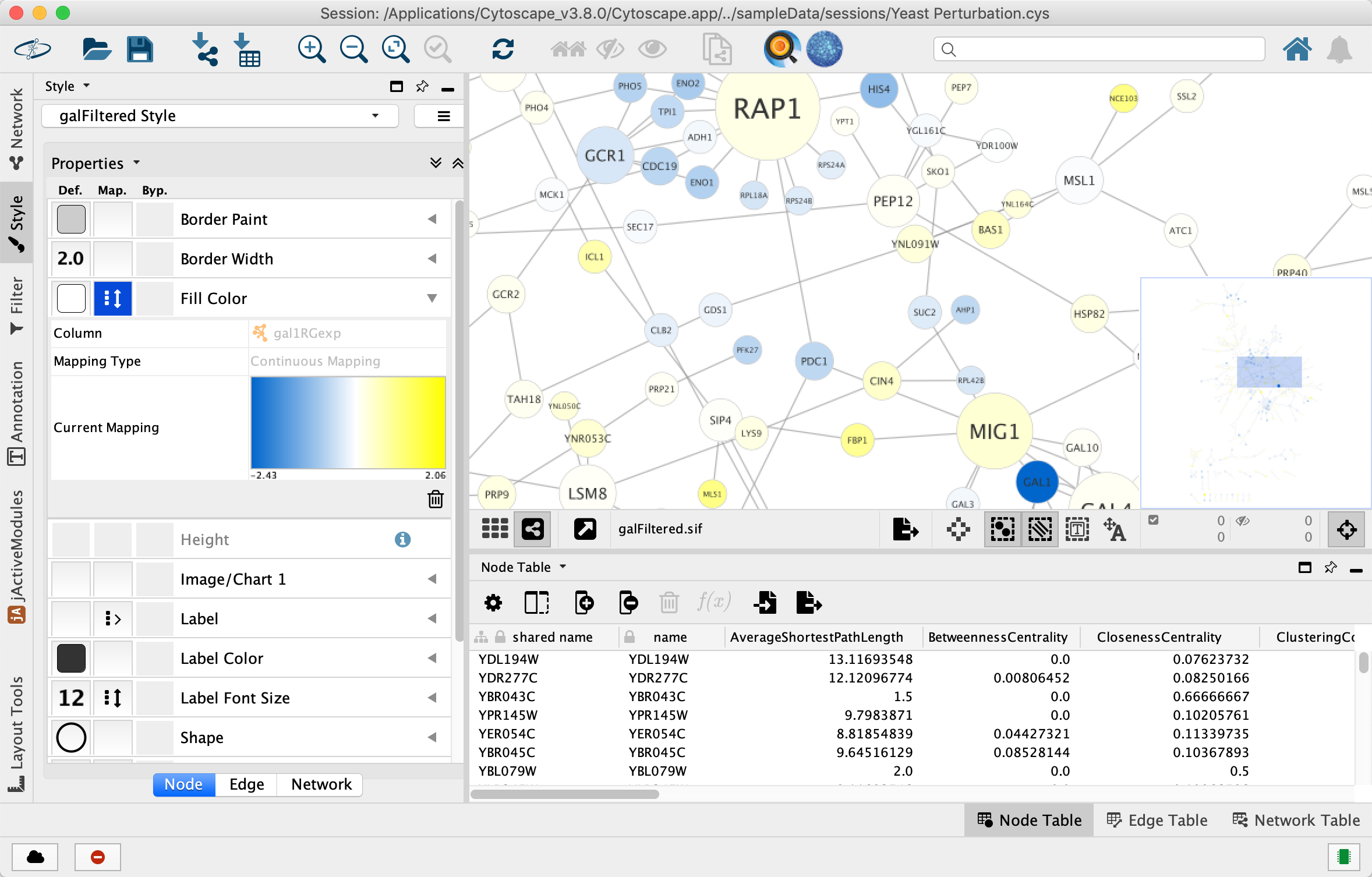
image
- Open source, cross platform Java desktop GUI app.
- for network visualization.
Why do we need to automate?
Why automate Cytoscape when I could just use the GUI directly?
- For things you want to do multiple times, e.g., loops
- For things you want to repeat in the future
- For things you want to share with colleagues or publish
- For things you are already working on in R or Python, etc
- To prepare data for collaborators
In short, for “reproducibility”, “data sharing”, “the use of R or Python”.
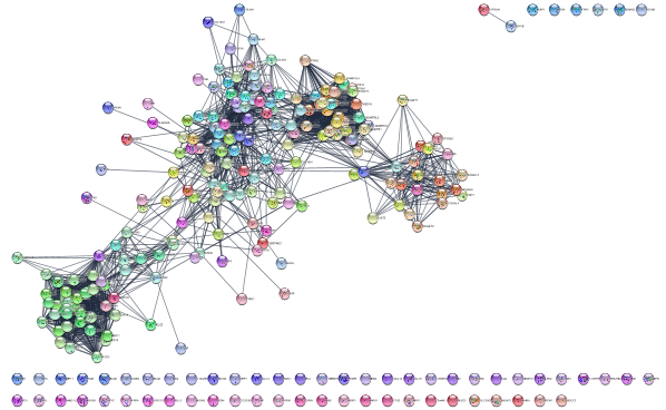
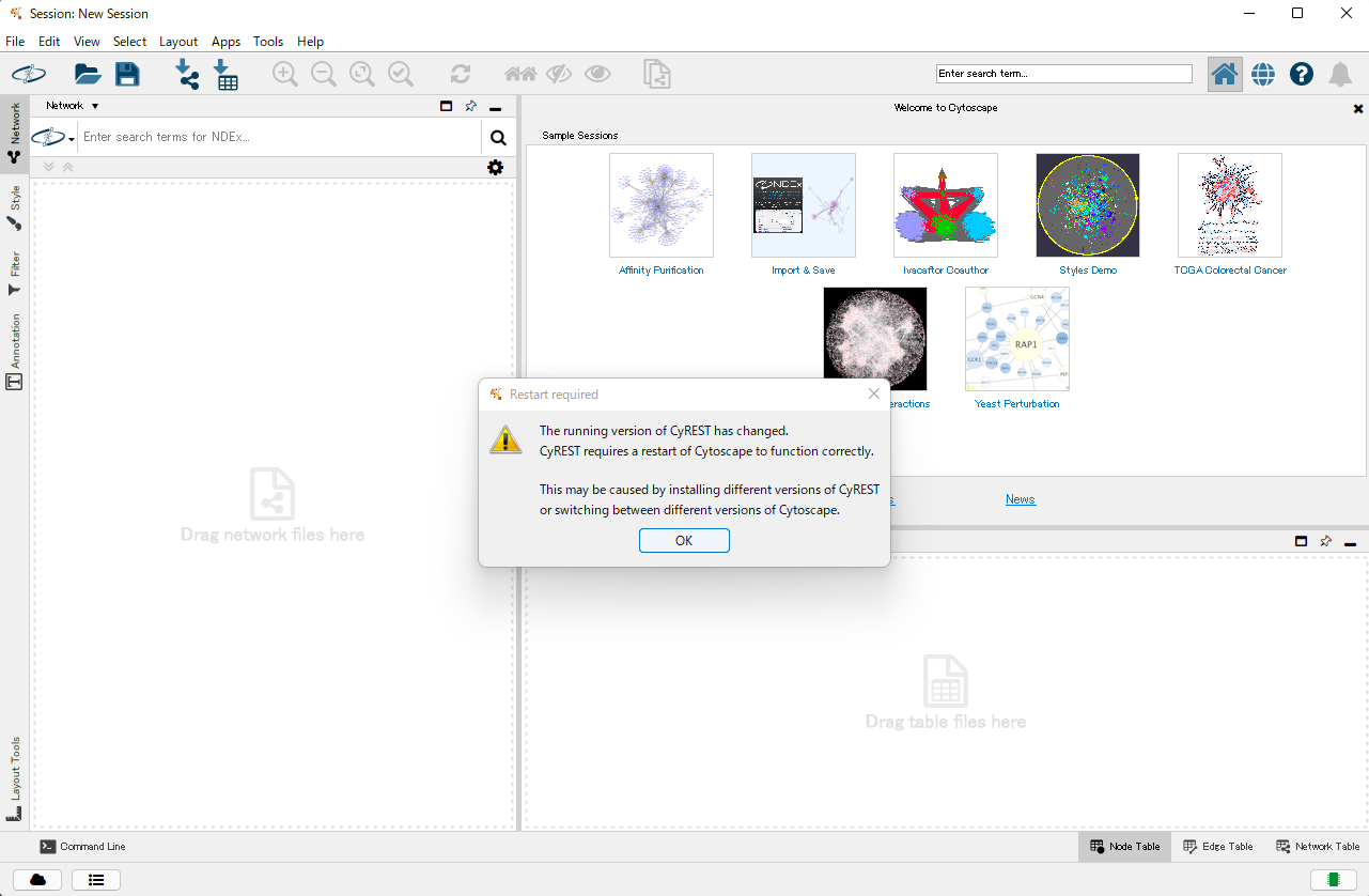
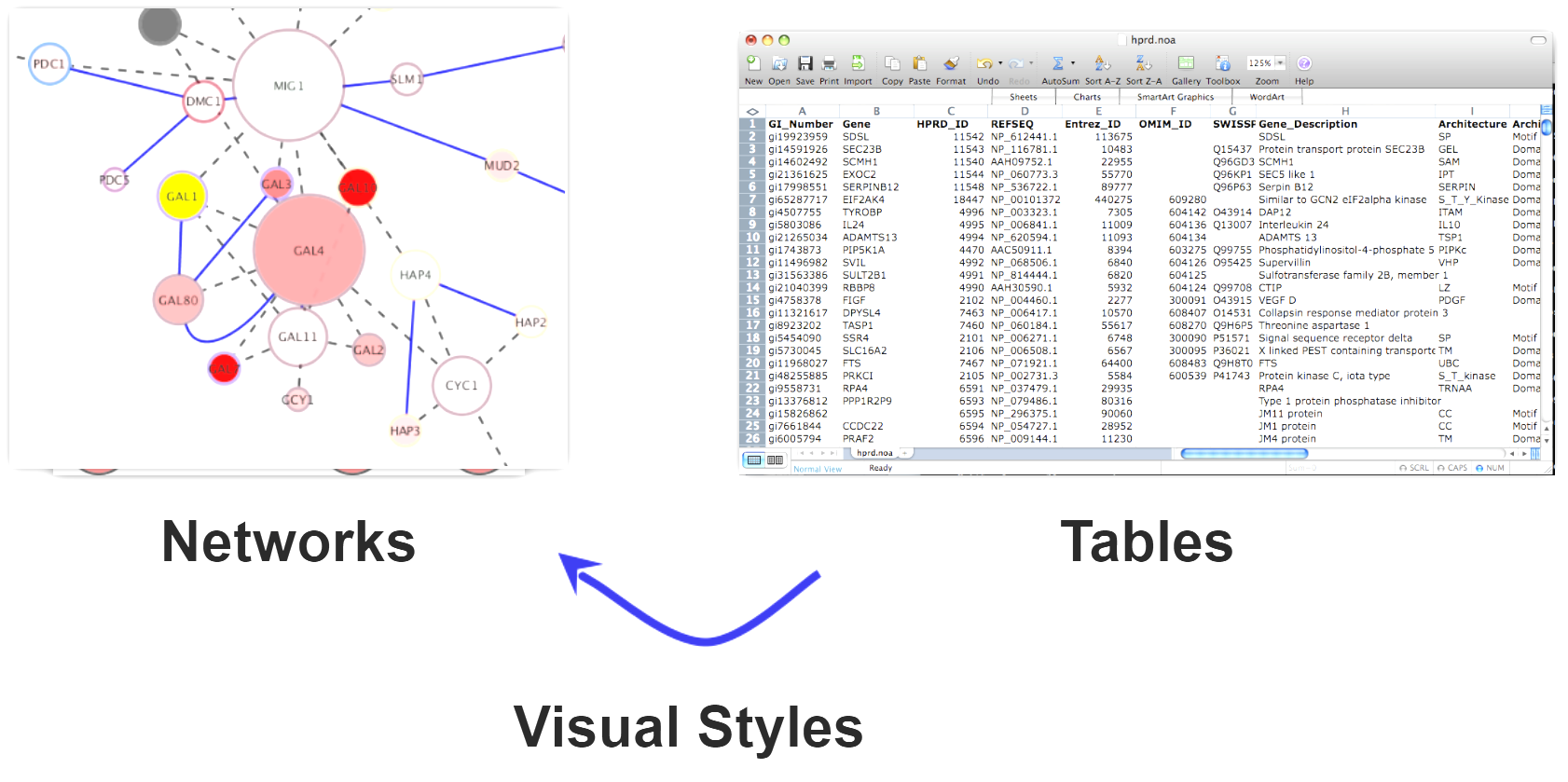
How can Cytoscape GUI operations be automated?

image
Cytoscape makes that possible with the REST API.
Today Cytoscape is not only a Desktop application but also a REST server.
-
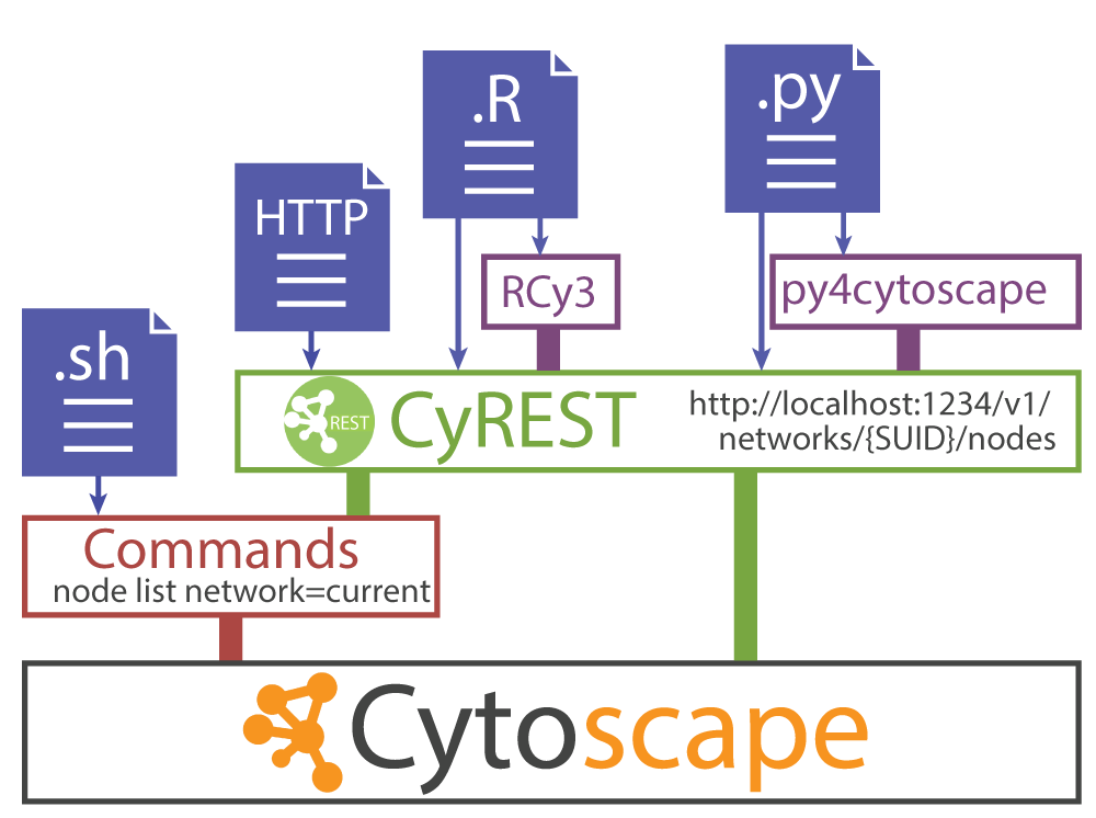
You can check if Cytoscape is now working as a server with the command below.
curl localhost:1234 -
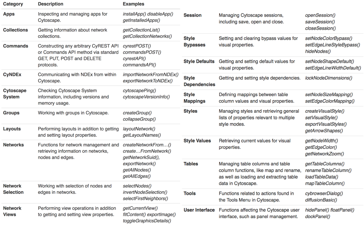
Now Cytoscape has REST API for almost every GUI operation.
- RCy3 or py4cytoscape is R or Python wrapper of the REST API
- py4cytoscape is Python clone of RCy3, py4cytoscape has same function specifications with RCy3
Since table operations are essential for Bioinformatics, it is convenient to be able to operate them with R[dplyr] or Python[pandas].
CyREST: Turbocharging Cytoscape Access for External Tools via a RESTful API. F1000Research 2015.
Cytoscape Automation: empowering workflow-based network analysis. Genome Biology 2019.
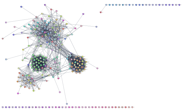
Translating R data into a Cytoscape network using RCy3
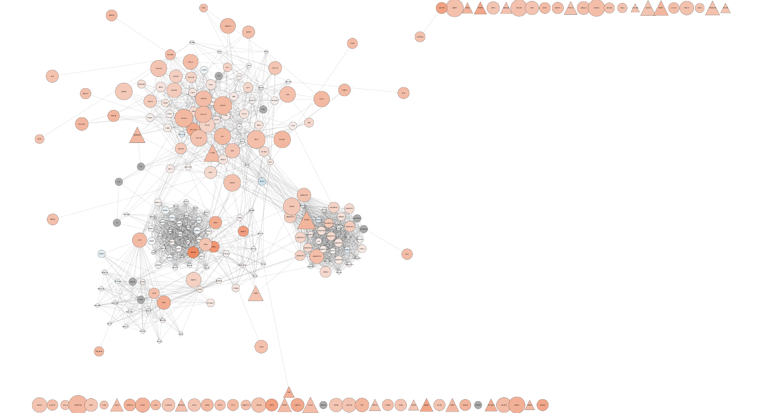
Networks offer us a useful way to represent our biological data. But how do we seamlessly translate our data from R into Cytoscape?
image
From here it finally becomes hands-on using Google Colab. Aside from the details, let’s connect Google Colab to local Cytoscape.
Make sure your local Cytoscape is fully up and running before running the code below. It will take some time for Cytoscape to start up and its REST server to start up completely. (Please wait for about 10 seconds.)
library(RCy3)
browserClientJs <- getBrowserClientJs()
IRdisplay::display_javascript(browserClientJs)
cytoscapePing()
Why was the remote Google Colab able to communicate with the local Cytoscape REST service?
We need a detailed description of what happened in
browserClientJs <- getBrowserClientJs()
IRdisplay::display_javascript(browserClientJs)
We used a technology called Jupyter Bridge in the above code. Jupyter Bridge is a JavaScript implementation that makes HTTP requests from a remote REST client look like local requests.
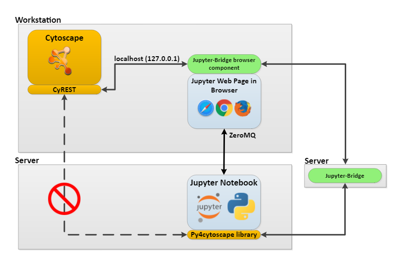
image
Since it is difficult to access Cytoscape in the desktop environment from a remote environment, we use Jupyter Bridge.
And since I couldn’t get Jupyter Bridge to work in the Orchestra environment, this workshop is exceptionally using Google Colab instead of Orchestra.
If you have RCy3 installed locally instead of remotely like Google Colab, you don’t need to use this Jupyter Bridge technology.
(Then) Why use Jupyter Bridge?
- Users do not need to worry about dependencies and environment.
- Easily share notebook-based workflows and data sets
- Workflows can reside in the cloud, access cloud resources, and yet still use Cytoscape features.
Let’s go back to how to translate R data into a Cytoscape network…
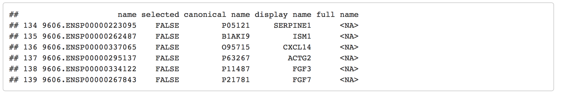
Create a Cytoscape network from some basic R objects
nodes <- data.frame(id=c("node 0","node 1","node 2","node 3"),
    group=c("A","A","B","B"), # categorical strings
    score=as.integer(c(20,10,15,5)), # integers
    stringsAsFactors=FALSE)
nodes
edges <- data.frame(source=c("node 0","node 0","node 0","node 2"),
    target=c("node 1","node 2","node 3","node 3"),
    interaction=c("inhibits","interacts","activates","interacts"),  # optional
    weight=c(5.1,3.0,5.2,9.9), # numeric
    stringsAsFactors=FALSE)
edges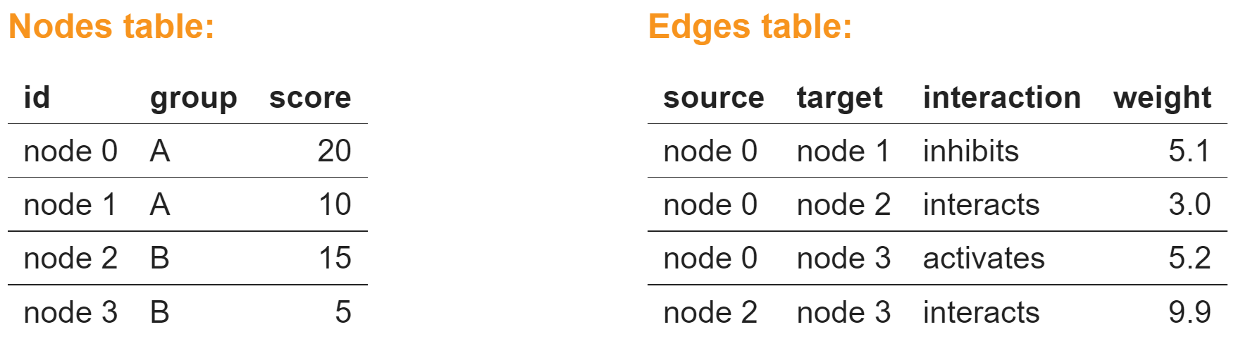
Create Network
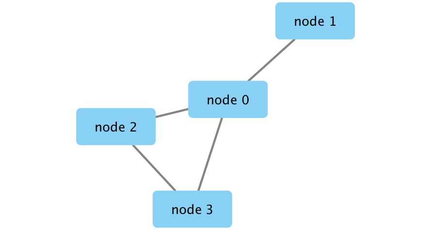
createNetworkFromDataFrames(nodes, edges, title="my first network", collection="DataFrame Example")Export an image of the network
Remember. All networks we make are created in Cytoscape so get an image of the resulting network and include it in your current analysis if desired.
exportImage("my_first_network", type = "png")Initial simple network
image